In the last years the use of microarrays as predictors of clinical outcomes (van 't Veer et al., 2002), despite not being free of criticisms (Simon, 2005), has fuelled the use of the methodology because of its practical implications in biomedicine. Many other fields, such as agriculture, toxicology, etc are now using this methodology for prognostic and diagnostic purposes.

Predictors are used to assign a new data (a microarray experiment in this case) to a specific class (e.g. diseased case or healthy control) based on a rule constructed with a previous dataset containing the classes among which we aim to discriminate. This dataset is usually known as the training set. The rationale under this strategy is the following: if the differences between the classes (our macroscopic observations, e.g. cancer versus healthy cases) is a consequence of certain differences an gene level, and these differences can be measured as differences in the level of gene expression, then it is (in theory) possible finding these gene expression differences and use them to assign the class membership for a new array. This is not always easy, but can be aimed. There are different mathematical methods and operative strategies that can be used for this purpose.

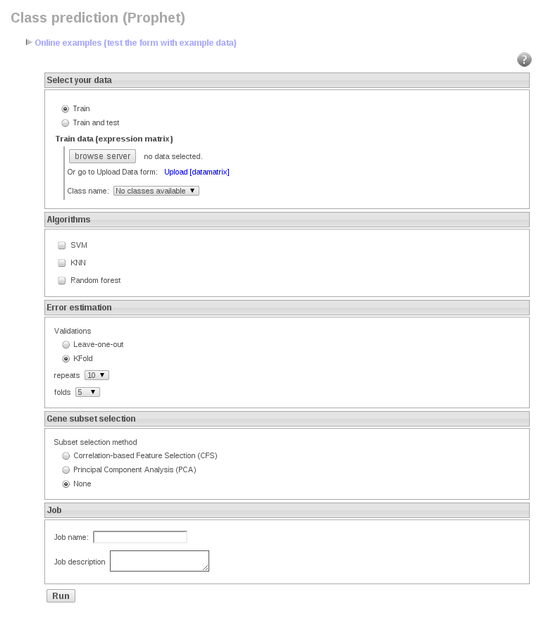
Prophet is a web interface to help in the process of building a “good predictor”. We have implemented several widely accepted strategies so as Prophet can build up simple, yet powerful predictors, along with a carefully designed cross-validation of the whole process (in order to avoid the widespread problem of “selection bias”).

Prophet allows combining several classification algorithms with different methods for gene selection.

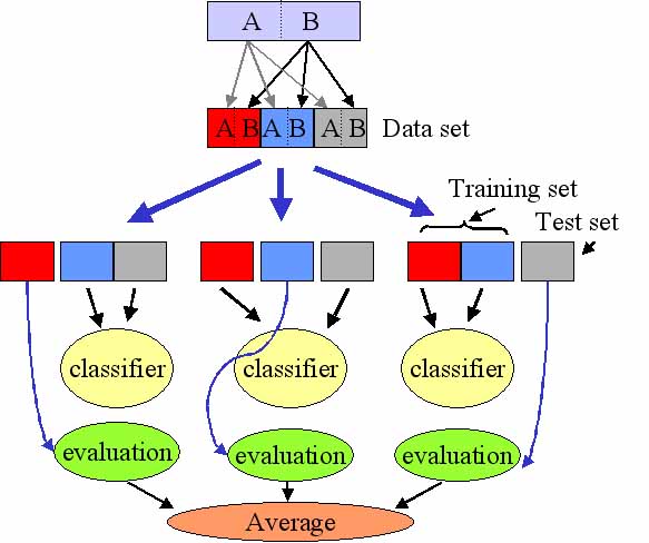
A predictor is a mathematical tool that is able to use a data set composed by different classes of objects (here microarrays) and “learn” to distinguish between these classes. There are different methods that can do that (see below). The most important aspect in this learning is the evaluation of the performance of the classifier. This is usually carried out by means of a procedure called cross-validation. The figure illustrates the way in which cross-validation works. The original dataset is randomly divided into several parts (in this case three, which would correspond to the case of three-fold cross validation). Each part must contain a fair representation of the classes to be learned. Then, one of the parts is set aside (the test set) and the rest of the parts (the training set) are used to train the classifier. Then, the efficiency of the classifier is checked by using the corresponding test set which has not been used for the training of the classifier. This process is repeated as many times as the number of partitions performed and finally, an average of the efficiency of classification is obtained.

Figure 1 - Cross validation

We have included in the program several methods that have been shown to perform very well with microarray data (Dudoit et al., 2002; Romualdi et al., 2003; Wessels et al., 2005). These are support vector machines (SVM), k-nearest neighbor (KNN) and Random Forest (RF).

• Support Vector Machines (SVM): Recently, SVM (Vapnik, 1999) are gaining popularity as classifiers in microarrays (Furey et al., 2000; Lee & Lee, 2003; Ramaswamy et al., 2001). The SVM tries to find a hyperplane that separates the data belonging to two different classes the most. It maximizes the margin, which is the minimal distance between the hyperplane and each data class. When the data are not separable, SVM still tries to maximize the margin but allow some classification errors subject to the constraint that the total error (distance from the hyperplane to the wrongly classifies samples) is below a threshold.

• Nearest neighbour (KNN): KNN is a non-parametric classification method that predicts the sample of a test case as the majority vote among the k nearest neighbors of the test case (Ripley 1996; Hastie et al., 2001). The number of neighbors used (k) is often chosen by cross-validation. (Ripley 1996; Hastie et al., 2001).

• Random Forest (RF): It is an ensemble classifier that consists of many decision trees and outputs the class that is the mode of the class's output by individual trees (Leo Breiman,2001)

In machine learning and statistics, feature selection, also known as variable selection, feature reduction, attribute selection or variable subset selection, is the technique of selecting a subset of relevant features for building robust learning models. When applied in biology domain, the technique is also called discriminative gene selection, which detects influential genes based on DNA microarray experiments

• Correlation-based Feature Selection (CFS), This method comes from the thesis of Mark A. Hall., 1999. This algorithm claims that feature selection for supervised machine learning tasks can be accomplished on the basis of correlation between features. In particular, this algorithm investigates the following hypothesis:

"A good feature subset is one that contains features highly correlated with (predictive of) the class, yet uncorrelated with (not predictive of) each other".

• Principal Components Analysis (PCA): involves a mathematical procedure that transforms a number of possibly correlated variables into a smaller number of uncorrelated variables called principal components. The first principal component accounts for as much of the variability in the data as possible, and each succeeding component accounts for as much of the remaining variability as possible. Dimensionality reduction is accomplished by choosing enough eigenvectors to account for some percentage of the variance in the original data, default 0.95 (95%). Attribute noise can be filtered by transforming to the PC space, eliminating some of the worst eigenvectors, and then transforming back to the original space.

After ranking the genes by PCA, we examine the performance of the class prediction algorithm using different numbers of the best ranked genes and select the best performing predictor. In the current version of Prophet we build the predictor using the best 5, 10, 15, 20, 25, 30, 35, 40, 45 and 50 genes. You can choose other combinations of numbers anyway. Note, however, that most of the methods require starting by, at least, 5 genes.

If the gene selection process is not taken into account in the cross-validation, the estimations of the errors will be artificially optimistic. This is the problem of selection bias, which has been discussed several times in the microarray literature (Ambroise & McLachlan 2002; Simon et al. 2003). Essentially, the problem is that we use all the arrays to do the filtering, and then we perform the cross-validation of only the classifier, with an already selected set of genes. This cannot account properly for the effect of pre-selecting the genes. As just said, this can lead to severe underestimates of prediction error (and the references given provide several alarming examples). In addition it is very easily to obtain (apparently) very efficient predictors with completely random data, if we do not account for the pre-selection.

The optimal number of genes to be included in a predictor is not know beforehand and it depends on the own predictor and on the particular dataset. A rather intuitive way of guessing about it is by building predictors for different number of genes (see above). Unfortunately, by doing this we are again falling into a situation of selection bias, because we are estimating the error rate of the predictor without taking into account that we are choosing the best among several trials (8 in this case).

Thus, another layer of cross-validation has been added. We need to evaluate the error rate of a predictor that is built by selecting among a set of rules the one with the smallest error.

The cross-validation strategy implemented here return the cross-validated error rate of the complete process. The cross-validation affect to the complete process of building several predictors and then choosing the one with the smallest error rate.

Here is a screenshot of the train interface.

The file with the gene expression values must be compliant with the Babelomics format, that is, rows represent genes, and columns represent arrays (samples, tissues, individuals, etc.) Array labels can be provided for easier interpretation of the results. To do that, add in the header of the file a line stating by “#NAMES“ or “#names“ and then list one label per array separated by tabulators.

Importants things to take into consideration:

• missing values are not allowed here. You can use the preprocessor for either get rid of them or imputing the values
• lines cannot end with a tabulator
• lines starting with #, distinct than “#NAMES“ or “#names“, will not be considered
• the first column must be the name of the gene or an id
• all values are separated by tabulators

An extra file defining the classes to which the arrays belong to must be provided.

Separate class labels by tab (t), and end the file with a carriage return or newline. No missing values are allowed here. Class labels can be anything you wish; they can be integers, they can be words, whatever.

All labels must be in one line. As before, the line can't end with a tabulator and the lines startong with # will not be considered

This is a simple example of class labels file

#VARIABLE TUMOR CATEGORICAL{ALL,AML} VALUES{ALL,ALL,ALL,ALL,ALL,ALL,ALL,AML,AML,AML,AML,AML} DESCRIPTION{}

In this example we are going to analyse a dataset from Golub et al. (1999). In that paper they were studying two different types of leukaemia (acute myeloid leukemia (AML) and acute lymphoblastic leukemia (ALL) in order to detect differences between them. This dataset have 3051 genes and 38 arrays, 27 of them labeled as ALL and 11 of them as AML.

Using Prophet we are going to build a predictor to try to distinguish between both classes. In the train file we can see 30 arrays, 22 ALL and 9 AML. The rest, 6 ALL and 2 AML, are in the test file for predicting.

You can find the dataset for this exercise in the following files:

• The first one is the file to train the predictor: datatraingolub.txt
• The second one will be used to predict the classes (test dataset): datatestgolub.txt

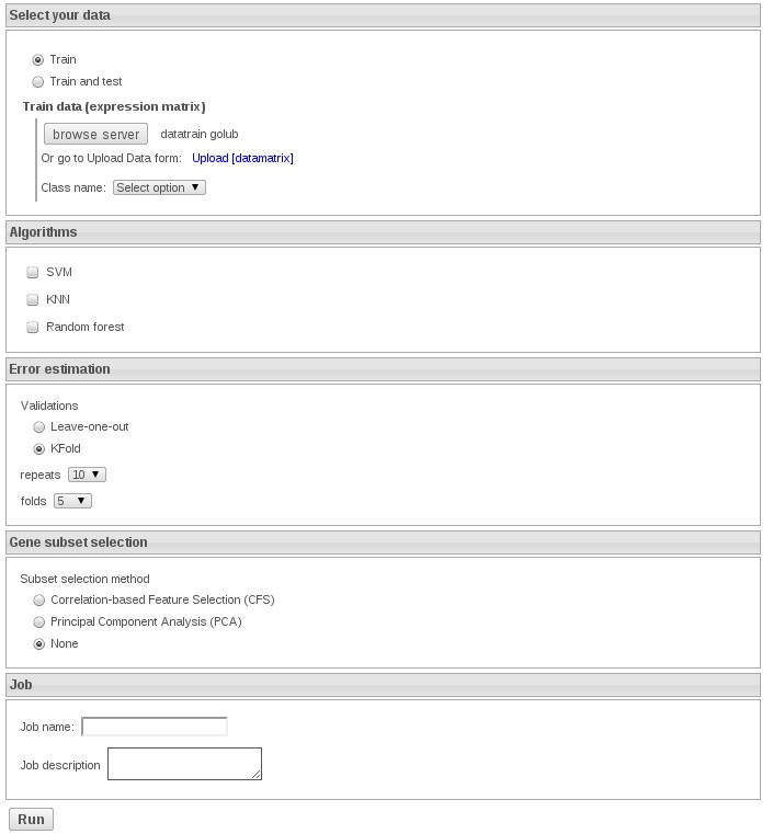
1) Train with knn: Upload the datafile and select the variable TUMOR

In order to get the exercises fast select 5 repeats of 5-fold cross validation. In this exercise do not select any feature selection method.

2) Repeat the exercise but select CFS feature selection method, which one works better? why? how many genes were selected

3) Now try with svm with no feature selection method, which one performs better? SVM or KNN

4) To finish you can try SVM with CFS feature selection method, how many features were selected? why it matches KNN with CFS?

5) Finally, which is the bes combination? why is SVM doing better alon than with CFS?

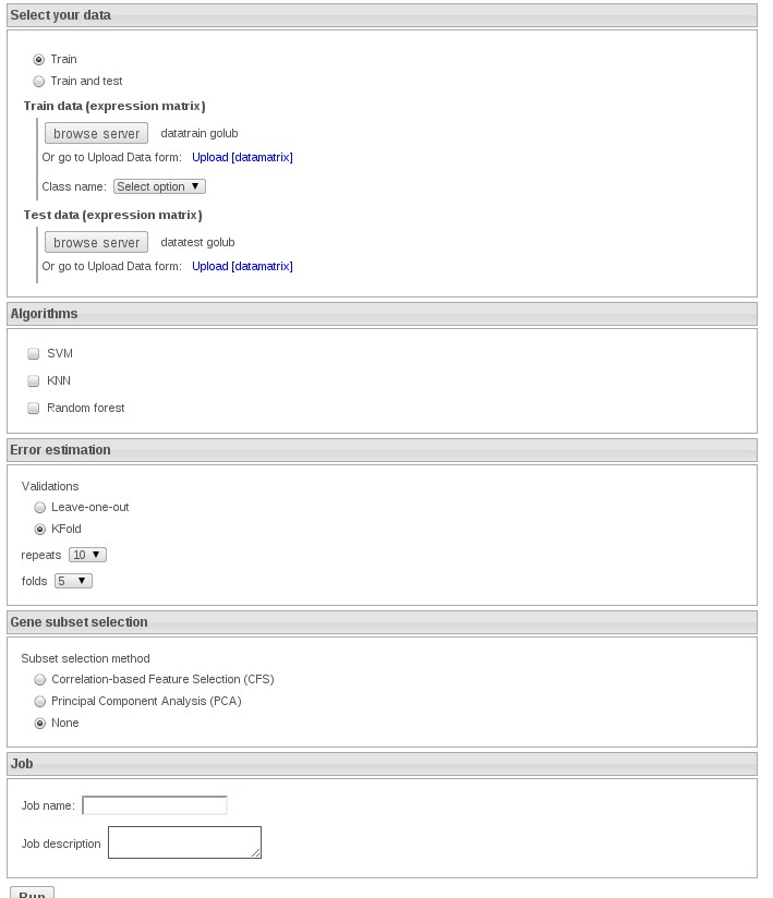
Now we select the option Train and test and select datatraingolub and datatestgolub:

We can select KNN without feaure method to speed up the exercise.

In order to check the accuracy of prediction you can see the correct labels for the test file:

ALL ALL ALL ALL ALL ALL AML AML

Are the predictions right? Do you get the same results with SVM?

• Ambroise, C. and McLachlan, G. J., (2002). Selection bias in gene extraction on the basis of microarray gene expression data. Proc Natl Acad Sci USA, 99:6562-6566.
• Breiman, L., 2001. Random forests. Machine Learning, 45:5-32.
• Dudoit, S., Fridlyand, J., and Speed, T. P. (2002). Comparison of discrimination methods for the classification of tumors suing gene expression data. J Am Stat Assoc, 97:77-87.
• Hastie, T., Tibshirani, R., and Friedman, J., (2001). The elements of statistical learning. Springer, New York.
• Lee, JW , Lee JB, Park M, Song SH (2005) An extensive comparison of recent classification tools applied to microarray data Computational Statistics & Data Analysis 48: 869-885
• van 't Veer, L.J., Dai, H., van de Vijver, M.J., He, Y.D., Hart, A.A., Mao, M., Peterse, H.L., van der Kooy, K., Marton, M.J., Witteveen, A.T. et al. (2002) Gene expression profiling predicts clinical outcome of breast cancer. Nature, 415: 530-536.
• Ripley, B. D. (1996). Pattern recognition and neural networks. Cambridge University Press, Cambridge.
• Simon, R. (2005) Roadmap for developing and validating therapeutically relevant genomic classifiers. J Clin Oncol, 23: 7332-7341
• Simon, R., Radmacher, M. D., Dobbin, K., and McShane, L. M., (2003). Pitfalls in the use of DNA microarray data for diagnostic and prognostic classification. Journal of the National Cancer Institute, 95:14-18.
• Tibshirani, R., Hastie, T., Narasimhan, B., and Chu, G., (2002). Diagnosis of multiple cancer types by shrunken centroids of gene expression. Proc Natl Acad Sci USA, 99:6567-6572.
• Vapnik, V (1999) Statistical learning theory. John Wiley and Sons. New York.
• Wessels LF, Reinders MJ, Hart AA, Veenman CJ, Dai H, He YD, van't Veer LJ(2005) A protocol for building and evaluating predictors of disease state based on microarray data. Bioinformatics.21(19):3755-62.