Babelomics' set of tools for differential gene expression analysis can be found in the Differential expression button of the Tools drop down menu. There are four different experimental contexts that you can explore using Babelomics:

1. You can find genes differentially expressed in a class, between two or more classes.

• Detecting expression patterns more differentiated between several two-colors arrays of the same class (one-class).
• It is possible with to study differential gene expression between two conditions. For example, when comparing tumor and healthy cells you can find which genes are over-expressed or under-expressed in the tumor compared to the healthy cells.
• Also, it is possible indeed, to analyze differential expression among more than two conditions. For instance, if you are studding three different types of tumor cells, you can find the genes that have expression patterns more differentiated among them.

2. Another kind of data that you can handle with our tools are those concerned with differential gene expression related to a continuous variable. For example, if you treat some cells with different doses of a drug and you also measure their gene expression levels, you can find genes which expression increases or decreases with the level of treatment.

3. Other analysis that can be done is to explore gene expression related to a survival time. You can study for example which genes are more directly related to the death of your cells by analyzing the relationships between the expression of the genes and the survival time of the cells.

4. Finally, you can also analyze time or dosage series. The module finds genes with a changing pattern along time or increasing dose concentrations, and with different profile evolutions between different series (i.e. treatments, strains, tissues, etc).

There are many different statistical approaches to the aforementioned scenarios. Babelomics implements some classical methodologies as well as some of the newer algorithms that are known to have enhanced performance in dealing with gene expression data.

Estimates for statistics and p-values are used to order genes in terms of their pattern of differential expression. When it is desirable, p-values adjusted for multiple testing are provided.

All your data are supposed to have been pre-processed and normalized before analyzing them with the differential gene expression module in Babelomics. For some microarray platforms you can do this using Babelomics' normalizing and pre-processing tools, but for some other you will need to use external software and then introduce the preprocessed data in Babelomics.

In general, missing_data are not allowed in your data. See the Babelomics' Preprocessing tool to deal with missing data and other data handling options.

The general structure assumed for your data is a numerical matrix of gene expression measurements. Measurements of the same gene are supposed to be in the same row while measurements under the same experimental condition (same array for instance) are assumed to be in the same column. That is, the data structure returned by the normalization module of Babelomics.

It is always necessary that the first column of the data file contains some gene identifier as for example the gene name. A general good practice when doing gene expression analyses is not to have duplicated gene identifiers. If there are several expression measurements for any of your genes you are responsible to know the reason why and how to deal with it, including so how to distinguish the replicated measurements. The Babelomics' pre-processing tool offers you some ways to manage such situations.

An example of expression data file with the above mentioned structure would look like this:

    gene1	10.23	9.98	10.41	10.55	10.65	9.69
    gene2	10.51	9.74	10.65	10.63	10.43	10.35
    gene3	9.89	10.02	9.89	11.03	10.21	10.77
    gene4	10.25	10.83	8.94	10.16	10.49	10.46
    gene...	...	...	...	...	...	...

Apart from the expression data some additional information is needed depending on the kind of analysis you are doing. In general this complementary information does not relate directly to the genes but to the experimental conditions. For example the class of the samples you are analyzing or the survival times of each cell culture are characteristic to all genes within one array.

You can insert such additional information in Babelomics Processing module. Here you have more information about editing variables.

As said before, Babelomics Differential Gene Expression module distinguishes among four conceptually different testing cases:

limma
This option allows us to detect genes with a significant gene expression (different to 0) between several two-colors arrays in the same experimental condition or class.
Limma is a package for the analysis of gene expression microarray data, especially the use of linear models for analysing designed experiments and the assessment of differential expression. This option estimates the variability of data using a diferent method. More information about limma package

The purpose of this set of tests is to study differential expression between two groups or classes of arrays. Just two classes are allowed in this set of tests. If you want to analyze more than two classes go to the multi class set of tests.

According to each test, genes are ranked from more expressed in one class (the first value of class variable in the form) to more expressed in the second one (the second and last one in your variable class) passing through no differentially expressed. You might find this arrangement useful in further studies, for example when trying to find sets of functionally related genes that are also differentially expressed using FatiGO or FatiScan for example.

t-test
This option performs, for each gene, a t-test for the difference in mean expression between the two groups of arrays. T-statistics and p-values are reported.
In the output file as well as in the image, genes are ranked according to the t-statistic. Genes in the top of the results list are those more expressed in your first class. Genes in the bottom part of the list are those more expressed in the second class. More information

limma
Interpretation of limma results is like t-test results.
Limma is a package for the analysis of gene expression microarray data, especially the use of linear models for analysing designed experiments and the assessment of differential expression. This option estimates the variability of data using a diferent method. More information about limma package

fold-change
Fold-change analysis is used to identify genes with expression ratios or differences between two classes that are outside of a given cutoff or threshold.
If you normalized data includes logarithmic transformation, you should calculate fold-change as the difference between means of two classes.
In another case, you can calculate fold-change as log2 of ratio between means of two classes.

The purpose of this set of tests is to study differential expression among more than two groups or classes of arrays. The methods implemented here allow you finding genes differentially expressed between more than two classes. If you want to analyze just two classes go to the two class set of tests.

While the mathematical treatment of this kind of data is similar to that of two classes, in our tools, we separate the case when more than two classes are available because of its conceptual implications. In the case of differential expression between two classes genes can be ranked from most expressed in the first class to most expressed in the second one, passing through non-differentially expressed genes. Such ranking of genes might have a straightforward biological interpretation as well as many advantages in terms of further analyses. However, when more than two classes describe our data, the ranking of genes by their differential expression is not straightforward and we need to be more cautious when interpreting the results

ANOVA
For each gene, this option performs a classical analysis of variance to test for mean differences between the array groups defined by the class labels. In the output file as well as in the image, genes are ranked by their estimated p-values, from more differentiated between groups to more similar among them.
More information

limma
Interpretation of limma results is like anova results.
Limma is a package for the analysis of gene expression microarray data, especially the use of linear models for analysing designed experiments and the assessment of differential expression. This option estimates the variability of data using a diferent method. More information about limma package

The purpose of this section is to study gene expression related to some continuous independent variable. We implement here some statistical methods that allow you finding genes whose expression is dependent on a continuous variable like for instance the level of a metabolite.

In the output file as well as in the image, genes are arranged first according to the sign of the correlation coefficient (or the slope in the case of regression analysis) and second by p-values. Genes in the top of the results list are those with stronger positive linear dependence of the explanatory variable. Genes in the bottom part of the list are those with negative linear dependence of the explanatory variable.

Pearson's test.
Pearson's correlation coefficient is computed between the intensities measured for each gene and the values of the independent variable. P-values to test for the null hypothesis that the correlation is zero are provided. More information

Spearman's test.
Calculation of the Spearman rank order correlation coefficient is performed. P-values to test for the null hypothesis that the correlation is zero are provided.
More information

Regression.
A regression analysis is performed for each gene; measured intensities being regressed on the independent variable. Estimates for the intercept and slope are provided together with the statistic and p-value to test for the null hypothesis that the slope is zero. More information

The purpose of this tool is studying gene expression as explanatory variable for survival times associated to each array. A Cox proportional hazards regression model is fitted for each gene. We report estimates of the regression coefficient modeling the hazard function (in the log scale). We also provide p-values to test for the null hypothesis that the coefficient is zero. More information.

In the results file an in the image, genes are ranked first according to the sign of the coefficient and second by p-values. Genes on the top of this arrangement are those for which high expression is associated to higher values of the hazard function (shorter survival times). In the bottom of the arrangement are allocated the genes for which high expression is associated to lower values of the hazard function (longer survival times).

maSigPro is a methodology for identifying differentially expressed genes in a time-course or dosage-response transcriptomic experiment. The basic requisite is that the experiment includes a variable (time/dosage) which is of quantitative nature and each array in the experiment can be assigned a value for this variable. I this is the only factor in the experiment, we talk of Single Series Data and maSigPro looks for genes with expression changes related to this factor. If, additionally, there is a second factor in the experiment, for example, treatment, tissue, strain, we talk of Multiple Series Data and maSigPro looks for differences between this second factor over the course of the continuous variable. For example, differences in the expression profile, over time, between treatment A and treatment B. maSigPro uses a regression modeling approach to address this problem. maSigPro reports expression changes considering the whole expression profile, does not compares pair-wise time points or dosage values. In doing so, maSigPro is more sensitive than pair-wise comparisons methods as it considers the dynamics of gene expression. For more info, please see the maSigPro paper

Input parameters
When the analysis has finished you will get a web page with links to the input parameters, to the results of the analysis and to some links to other Babelomics tools that you can use to carry on with a meaningful analysis.

Output files
In the output file link you will find a text file with results of the analysis. In general this file will have a first column of gene identifiers followed by some more columns of estimate statistics, their respective p-values, raw and corrected (see multiple testing section) and some other results. Since each particular statistical method reports different parameters, the exact layout of the results file depends on the method that you applied to your data.

The way genes are ordered in the results files is thought to be statistically meaningful according to the method used in the analysis. It also tries to be most meaningful for the biological interpretation of the results. See the methods section for information about the arrangement of genes returned by each statistical test.

Images
In any analysis you run, we will provide a grid image representing your data. Each gene is represented in a row and each condition or array is represented in a column. High intensity measurements of gene expression are represented in red colors while blue colors represent lower measurements. Genes are sorted according to their expression patterns in the same order as they are in the output file. Experimental conditions or arrays are ordered depending on their labels.

When studying differential expression under two or more conditions arrays are sorted by class. The first class on the left will be the one that appears first in the specified value of class variable. The second class on the left will be the second one to appear in the selected values of class variable.

When analyzing correlation between expression and a continuous variable, arrays are arranged by the values of the continuous variable.

When performing survival analysis columns are arranged by the survival times.

Download the data from the Rheumatoid Arthritis dataset. Open the file with a text editor and see how it looks like. This data correspond to 15 samples from two conditions: disease and control.

Affymetrix (GeneChip Human Genome U95A Array) platform was used to do the hybridization. The data here presented have been normalized using rma methodology implemented in Babelomics normalization tools.

The original data, including .CEL files and information about the samples, can be downloaded from GEO. They correspond to the series GEO GSE1919.

We want to analyze differential gene expression between disease and control. To do this kind of analysis you can use the two-class section of the Babelomics Differential Gene Expression module.

Two steps:

1. Upload data.
Here you can upload data. Data type is “Data matrix expression”.

2. Go to the two-classes section of the Babelomics /Expression/Class comparison choosing:
- select your data: arthritis_rma.txt.
- select the class to analyze: arthritis (this variable differenciate two groups: 0 is control, 1 is disease).
- select test: ttest.
- select multiple test correction: FDR.
- select adj. p-value: 0.005.
- Name your job and running!

You will get a graph like this:

This option performs, for each gene, a t-test for the difference in mean expression between the two groups of arrays. T-statistics and p-values are reported.

In the output file as well as in the image, genes are ranked according to the t-statistic. Genes in the top of the results list are those more expressed in group 0 (control). Genes in the bottom part of the list are those more expressed in the group 1 (disease).

Download the data from the Molecular Apocrine Breast Tumor dataset. Open the file with a text editor and see how it looks like. This data correspond to 49 tumors of breast cancer patients. The tumors are classified into 3 classes: apocrine, basal and luminal.

Affymetrix (GeneChip Human Genome U133 Array Set HG-U133A) platform was used to do the hybridization. The data here presented have been normalized using rma methodology implemented in Babelomics normalization tools.

The original data, including .CEL files and information about the samples, can be downloaded from GEO. They correspond to the series GSE1561.

Imagine that we were now interested in finding the genes which expression pattern is more heterogeneous across all three tumors. Such genes could be the ones involved in the processes that differentiate the tumors behavior, having therefore a clinical interest.

To do this kind of analysis you can use the multi-class section of the Babelomics Differential Gene Expression module.

If you upload the data in Babelomics and you use the multi-class section of the Babelomics /Expression/Class comparison choosing the anova method, you will get a graph like this:

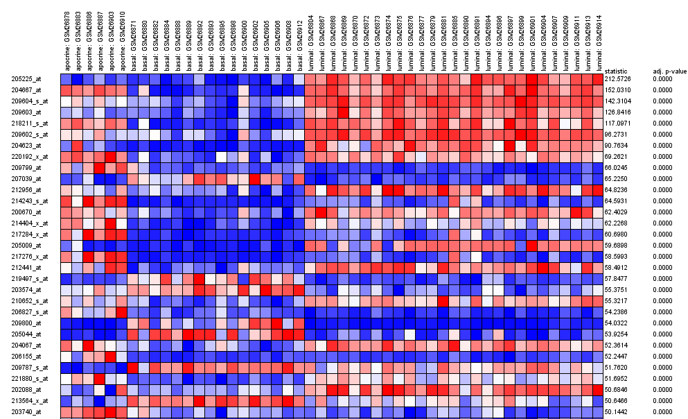
As in the two classes analysis, rows of the grid represents genes and columns represent arrays. In the columns of the right of the table you have the estimates of the F-statistic and the adjusted p-values (FDR).

Genes are ranked according to the significance of the differential expression among groups. Genes on the top of the table are those with more differentiated pattern across tumors. Genes on the bottom of the table are those showing less different pattern between tumors. If you see the results file you will see that genes are ranked in the same way they are in the graph. The results of Babelomics Differential Gene Expression module in this case arranges the genes from more differentially expressed among the classes to no differentially expressed among them.

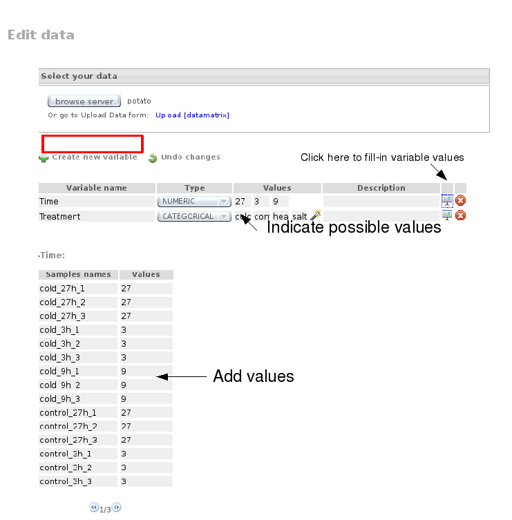
The study investigates the transcriptional response to three different abiotic stressors (Salt, Cold and Heat) in potato seedlings using the NSF 10k potato array See reference. A common reference design is used. The data set contains 4 series (1 Control and 3 types of stress: Heat, Salt and Cold), 3 time points, three replicates per experimental condition and 9124 genes.

Upload Data
The data for this example can be obtained here
Upload this dataset into Babelomics. Go to Data Upload, choose Expression-Matrix as data format and give it the name 'Potato'.
Go then to Data Preprocessing, select the Potato file, create two new variables, Time and Treatment, and assign corresponding values to each array:

Launch Job
Go to Expression → Time/dosage series.
Select the data “Potato” and Time and Treatment as Continuous and Series variable names, respectively. Since there are three time points in this example, we will select a polynomial degree 2. Leave the rest of the options default, write and job name and launch the job.
Once the analysis is completed you can go to the results page.
Results
Here you can see the basic maSigPro output: a list of differentially expressed genes for each comparison between Control and each Treatment, together with the Groups plot, in which genes are first divided into clusters of similar profiles and then represented as informative trajectory plots. By clicking on the comparison name, you obtain a file with the name of the significant genes and the cluster assignment. For example, cold_vs_control contains 2081 differentially expressed genes, distributed into 9 clusters see here . The “STMCB03 1” means that significant gene STMCB03 belongs to the cluster 1 visualized in the corresponding Groups Plot.

These lists can be sent to enrichment analysis to the FatiGO tool.

Another interesting plot is the Profiles Plot, where you can see the consistency of expression profiles for significant genes belonging to a given cluster. For example, if we look at the Profiles Plot os Cluster 1 in the cold.vs.control comparison, we observe a highly correlated pattern.

• Download the data from here. Open the file with a text editor and see how it looks like.

• This data corresponds to 12 samples of human tissue. They were taken from 6 healthy men, aged from 56 to 76, before and after 3 months of physical training.

• Affymetrix (GeneChip Human Genome U133 Array Set HG-U133A) platform was used to do the hybridization. The data here presented have been normalized using rma as implemented in Babelomics Affymetrix Normalization Tools.

• The original data, including .CEL files and information about the samples, can be downloaded from the NCBI repository called Gene Expression Omnibus. They correspond to the series GSE1786.

1. Use the data of this example to compare the samples of sedentary men with the trained ones. Use the t-test method and see the results file.
- Can you find any gene differentially expressed between the two groups?
- What is the implication of the sign of the estimate of the t-statistic?
- How is the relationship among the estimate of the statistic, the p-values and the adjusted p-values?

2. Use limma method to perform the same analysis. (Input parameters. Adj.p-value: 0.05 and Multiple-test correction: FDR)
- Compare the ranking of the genes given by the different methods. Are they very different?
- How many significant genes do you have?
- Change the adj.p-value: 0.1, using “Other actions/Open input form” from the form. Now, how many significant genes do you have?
- Redirect some of the results to FatiGO or FatiScan (the only parameters you need to select is the “Homo sapiens” label in the Organism box and some biological database, for example “GO Biological Process”). Don't worry! We will see these interesting functional tools in the next session.

3. Suppose that we are interested in finding genes which expression is higher or lower in elderly men than in young men.
- What tool do you have to use in Babelomics to evaluate the relationship between the expression of the genes and the age of the men?
- Use different tests. How is the arrangement of the genes in the heatmap?

• This is dataset that we used in the worked example 2.

1. Before we used anova test to evaluate expression gene between experimental conditions. Repeat the analysis using limma test. (Input parameters. Adj. p-value: 0.01, multiple test correction:FDR)
- How is the arrangement of the genes in the heatmap?
- How many significant genes do you have?
- Can you indicate the ten genes more differentially expressed? What does it mean in our experimental context?

2. Now, we are interested in comparing theses conditions by pairs. (Input parameters: adj. p-value: 0.01, multiple test correction:FDR)
- Compare the basal tumors with the luminal ones. How many genes do you have?
- Can you indicate the ten genes more under-expressed in luminal? And the gen more over-expressed in luminal?
- Compare the basal tumors with the apocrine ones. How many genes do you have?

• Download the data from here. Open the file with a text editor and see how it looks like.

• This time course study corresponds to 16 samples of a Human cell culture under different environmental conditions. Here you have more information relative to experimental design.

• One-color Agilent arrays were used. The data here presented have been normalized using Agilent background correction and quantiles between array normalization. Implemented methods in Babelomics.

1. We want to compare gene expression between treatment and control series over time. We can use Time/Dosage Series.
(Input parameters. Continuous variable: timeindays, name of variable defining series: class, significance level: 0.05, multiple testing adjustment: FDR, clustering: k-means, number of clusters: 9)
- How many genes have a significant changing profile between any of the treatment respect to control?
- Inspect the groups and profiles plots of the treatment vs. control. What can you say of the expression pattern represented Cluster 1? And of its homogeneity? What about cluster 3?
- Could we use a polynomial of degree 4 in this dataset?

Bolstad, B, Irizarry, R, Astrand, M, & Speed, T. (2003). A comparison of normalization methods for high density oligonucleotide array data based on variance and bias. Bioinformatics, 19(2), 185-193. doi: 10.1093/bioinformatics/19.2.185.

Benjamini, Y, & Hochberg, Y. (1995). Controlling the False Discovery Rate: A Practical and Powerful Approach to Multiple Testing. Journal of the Royal Statistical Society. Series B (Methodological), 57(1), 289-300. doi: 10.2307/2346101.

Benjamini, Y, & Yekutieli, D. (2001). The control of the false discovery rate in multiple testing under dependency. The Annals of Statistics. Volume 29, Number 4, 1165-1188.

Smyth GK. (2004). Linear Models and Empirical Bayes Methods for Assessing Differential Expression in Microarray Experiments. Statistical Applications in Genetics and Molecular Biology, 3(1). doi: 10.2202/1544-6115.1027.

Conesa A, Nueda MJ, Ferrer A, Talon M. (2006)“maSigPro: a method to identify significantly differential expression profiles in time-course microarray experiments.” Bioinformatics,22:1096-102.

http://www.bioconductor.org/