Different genes have different expression levels according to their specific function at each condition. Biclustering identifies groups of genes with similar expression patterns under a specific subset of conditions. These conditions may correspond to different time-points, for example in times series expression data.
The general structure of biclustering input data is a numerical matrix of gene expression measurements. Measurements of the same gene are supposed to be in the same row while measurements under the same experimental condition (same time point for instance) are assumed to be in the same column.
The first column of the data file must have some gene identifier as for example the gene name, and the first row of your data must have some time point identifier. Note that the word GENES should be in the first column and the first row without any comment symbol.
An example of biclustering input data file with the above mentioned structure would look like this:
    GENES    condition1    condition2    condition3    condition4    condition 5
    YAL001C  -0.19         -0.77         -0.17         -0.19         0.13
    YAL002W  0.83          -0.01         -0.77         -0.62         0.14
    YAL003W  -0.36         -0.22         0.22          -0.28         0.41
    YAL004W  1.64          1.14          0.88          -0.07         0.03
    YAL005C  1.55          1.58          1.34          0.01          0.53
    ...      ...           ...           ...           ...           ...
You can select different options of how biclustering analysis should deal with missing values.
Within type of missing values list there are the following options:
Remove: it deletes the complete gene row if this gene has a missing value.
Jump: it deletes the complete gene row if it affects the bicluster. Selected option by default.
Fill: it assigns a value where a missing value is found. There are different methods to assign this new value:
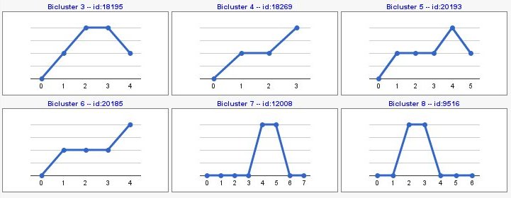
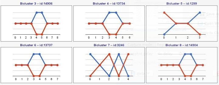
You can also compute patterns of opposite sign with 'compute sign changes' option. By default, this option is not selected and your pattern results would be as the following image,
Computing sign changes would give you patterns with both signs as you can see in the following example,
Biclustering results would be sorted by different criteria:
Genes: number of genes.
Time points: number of conditions.
Size: number of genes and number of conditions.
P-value: bicluster p-value. Selected option by default.
Biclustering results could be filtered by different criteria:
Constant patterns: it would not obtain those patterns in which genes do not change over time or conditions.
Minimum number of genes: it computes those biclusters with at least a minimum number of genes.
Minimum number of time points: it computes biclusters with at least a minimum number of conditions.
Maximum p-value: it computes biclusters with a maximum p-value.
Minimum overlapping percentage: it computes biclusters with a minimum percentage of overlapping between biclusters.
Go to the Babelomics page and select Biclustering analysis from the Expression menu.
Press Online Examples, select the example number 1 and you will see how the parameters and form fields are now filled. As you can notice, this example is prepared to perform a biclustering analysis with default parameters but filters. Selected filters are a minimum of 5 conditions and a maximum p-value of 0.05.
Press run, and wait for your job to be finished.
When the process finishes, a new green job is shown at the right side of the web page. Press it to check your results.
Results
Visualization of the results would be as the following image,
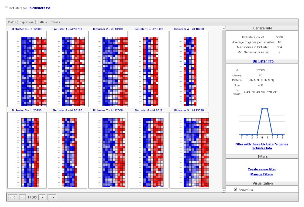
Biclusters file has information about all results, including a numerical matrix of expression measurements corresponding to the selected genes in each bicluster.
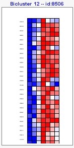
In the main box of the visualization tool, you would see obtained biclusters. Within the top menu you could change how to visualize them,
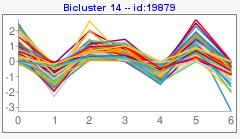
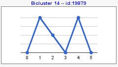
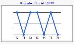
At the menu on the right there is a section with general information about the biclustering analysis, a section with information of a selected bicluster, a section where you can manage different filters and a visualization section.
Pattern coding is the following,
Questions
How many biclusters did you obtain?
In these results, which is the minimum number of genes that you find in a bicluster? and the maximum number of genes?
Select the pattern view at the top menu of the visualization box. Then, select the first bicluster (id:18191). How would you interpret this graph? What is your answer based on?
Select the trend plot of this bicluster. Is it different from its pattern plot?
In general, which are the differences between pattern plots and trends plots?
Run the same example with different options from the Babelomics interface. Compare the results.
Go to the Babelomics page and select Biclustering analysis from the Expression menu.
Press Online Examples, select the example number 2 and you will see how the parameters and form fields are now filled. As you can notice, this example is prepared to perform a biclustering analysis with remove missing values, compute sign changes and filter biclusters with a minimum of 5 conditions and a maximum p-value of 0.05.
Press run, and wait for your job to be finished.
When the process finishes, a new green job is shown at the right side of the web page. Press it to check your results.
Questions
How many biclusters did you obtain?
In these results, which is the minimum number of genes that you find in a bicluster? and the maximum number of genes?
Go to page 2 of results and select the bicluster with id:85. Then, click on 'Bicluster info' in the right menu. Are there any differences between derivative and trend patterns? What do those differences mean? In both patterns, how are gene expression values?
Send this bicluster to FatiGO analysis. Are its genes functionally enriched?
Then, click on 'Filter with these bicluster's genes' in the right menu. You will see a panel to insert genes that will filter biclustering results. Click on 'Show filter preview'. In how many biclusters are your list of genes? Which percentage of genes do you have in your list? Modify your list of genes and preview your filter.
Click on 'Filter' to obtain your filtered biclusters. If you want to manage and navigate through different filters, click on 'Manage filters' in the 'Filters' section of the rigth menu.
-
Madeira SC, Oliveira AL (2009)
A polynomial time biclustering algorithm for finding approximate expression patterns in gene expression time series.
Algorithms for molecular biology 4:8.
-
A.P. Gasch, P.T. Spellman, C.M. Kao, O. Carmel-Harel, M.B. Eisen, G. Storz, D. Botstein, and P.O. Brown (2000)
Genomic Expression Programs in the Response of Yeast Cells to Environmental Changes.
Molecular Biology of the Cell vol. 11, pp. 4241-4257.
S. Tavazoie, J.D. Hughes, M.J. Campbell, R.J. Cho and G.M. Church (1999)
Systematic Determination of Genetic Network Architecture.
Nature Genetics vol. 22, pp. 281-285.